| |
|

|
Step 1: |
|
Set up the position control system as it was in Part 2 of Experiment
7.3.
Verify that it still works.
Be sure to stop the controller program.
|
Step 2: |
|
Connect A/D input 3 (pin 4 on the interface board socket strip)
to  (the output of the summing amplifier).
|
Step 3: |
|
Load and run the "Calibrate" Labview program.
This will find the
actual range of  and the
actual values of
and the
actual values of  required at each
end of the range.
required at each
end of the range.
|
Step 4: |
|
When the Calibrate program has finished, write down the values
for
Vdrive hi,
Vdrive lo,
and
Vact lo.
|
Step 5: |
|
Load the "Controller 3" Labview program.
This is just like the "Controller 2" program, but it allows
for calibration, and also displays the error.
|
Step 6: |
|
Enter the values for
Vdrive hi,
Vdrive lo,
and
Vact lo
into the the appropriate fields on the control panel.
|
Step 7: |
|
Run the program and verify its operation.
|
| |
|
|
Step 1: |
|
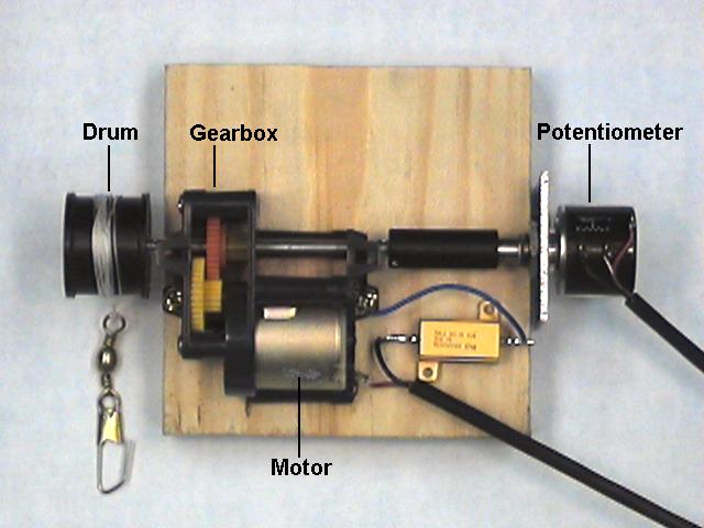
With the power to the motor turned off,
put the hook of the spring balance through the hook on the cord
wrapped around the drum.
|
Step 2: |
|
Slowly pull upward on the spring balance until the drum starts
to turn.
The highest value of force read on the balance before the drum turns
is the
static Coulomb friction,
the amount of force which must be applied before any motion can
take place.
Record this value in your lab notebook.
|
Step 3: |
|
Turn the power back on and restart the "Controller 3" program.
|
Step 4: |
|
Set the
Desired Position
control to -2.5.
|
Step 5: |
|
Manually turn the spool until the
Error
indicator reads zero.
|
Step 6: |
|
Slowly raise the
Desired Position
until the spool moves.
Note the value of the
Error
and
Vdif
just before
it moves.
|
Step 7: |
|
Slowly lower the
Desired Position
control until the spool moves again.
Again, note the values of
Error
and
Vdif
just before the motion takes place.
The difference between the two values of error is the
hysteresis
in the mapping of desired to actual position.
|
Step 8: |
|
Replace  (the 220k feedback resistor in the summing amplifier)
with values of 470k, 1M, 2.2M and 4.7M.
For each value, repeat the measurement of hysteresis.
(the 220k feedback resistor in the summing amplifier)
with values of 470k, 1M, 2.2M and 4.7M.
For each value, repeat the measurement of hysteresis.
|
Step 9: |
|
Plot the hysteresis vs.
.
|
Question 1: |
|
Explain the behavior of
as the gain is changed.
|
One way around this is to measure the average error with the system
in motion.
If we do this both going up and going down, the effects of friction
should cancel, leaving us with the error caused by the weight of the
load.
| |
|
|
Step 1: |
|
Load the "Ramp Response" Labview program.
This will run the hook down and back up at a constant rate, while
measuring the difference between the commanded position and the
actual position.
|
Step 2: |
|
Enter the calibration values for
Vdrive hi,
Vdrive lo,
and
Vact lo
into the the appropriate fields on the control panel.
|
Step 3: |
|
We will be measuring this error both as a function of the load
and as a function of the loop gain, as determined by
.
Make two tables, one for average error and one for peak error.
Allow for weights of 0, 1, 2, 3, and 4 oz
and for values of
of 220k, 470k, 1M, 2.2M, and 4.7M.
|
Step 4: |
|
With
set to 220k and no weights on the hook, run the program.
If all is well, the hook will lurch to the top, slowly run down, then
slowly run back up.
When this is finished, the program will display a plot of the actual
trajectory, the error as a function of time, and two numbers:
the average error
and the maximum error.
Record these values in your tables.
|
Step 5: |
|
Repeat the measurement with 1, 2, 3, and 4 ounce weights on the hook.
Also make printouts of several representative plots for your
notebook.
With the 4 oz. weight it is likely that nothing will happen.
With the 3 oz. weight you may get erratic performance.
If so, try several times and record the best measurement.
|
Step 6: |
|
Repeat the previous two steps with values of
of
470k, 1M, 2.2M, and 4.7M.
|
Step 7: |
|
Make a plot showing the average error vs. load for each value
of
.
Make another showing the average error vs.
for each
value of load.
|
Question 2: |
|
What is the expected behavior of the error in position as a function
of the weight of the load and of the controller gain A
?
Do your measurements support this expectation?
|